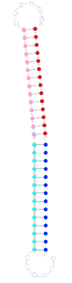
The repressive switches work in the reverse order to the activating switches. In the absence of triggers the RBS is accessible and therefore the switch is 'on'. Trigger binding draws the switch strand shut over the RBS by creating a hairpin.
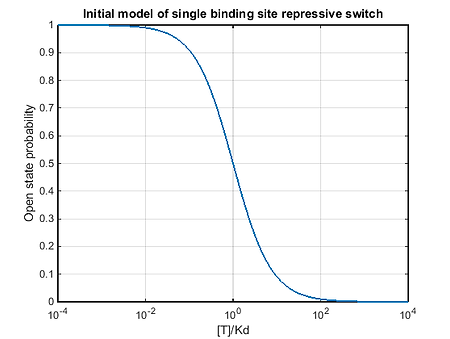
As the hairpin structure has a complex directionality, referred to as a pseudo-knot, it could not be simulated in Nupack. Our initial model for the mechanism of the repressive switch was similar to the activating switches, but with the reciprocal of all trigger dependent rates. The open state probability of the single binding site repressive switch was to be given by the following equation.
This model did not match experimental data (see in vitro repressive). We saw that the repressive switches were acting much more like activatory switches, increasing the open state probability with increasing trigger concentration.
The activatory behaviour of the repressive switches can be explained by the following 4 state model. In the repressive designs each end of the trigger binds to a separate binding sequence on the switch. If another trigger binds at the other half of the initial trigger's binding site then all of the sites will be used up, but the switch will not be drawn closed.
In the model of this process below, there are 4 states. The first, in which the switch is free, the second in which the first half of the trigger has bound to the switch, the third which is the desired hairpin structure, and, the fourth in which another trigger has mischievously bound to the remaining binding site.
These differential equations are solved in the steady state to calculate the probability that the switch is in an open state ( P(Open) = 1 - P(Closed) ) at a given trigger conc, [T].
The dissociation constants are defined as K1 = k21/k12, K3 = k32/k23, K4 = k42/k24.
The figure above is a plot of the open state probability for the repressive switch model for K1 = 0.001, K3 = 10, and K4 = 1. Accounting for the extra trigger binding event in the model confirms what was seen experimentally, that at high trigger concentrations the open state probability is not 0. Due to the pressure of excess triggers, in the high trigger concentration regime the repressive switch can have activating behaviour.
The heterotopic switches contain two different trigger binding sites, and respond to two different triggers, T1 and T2. In function they are similar to the homotropic switches, but now the degeneracy of the intermediate state is lifted. One trigger must bind before the other, and therefore there are two orders in which the switch can open. The binding of the first trigger destabilises the stem. The second trigger can bind to its binding site, and this stabilises the system in an open conformation.
The conformations of switch and trigger shown below were shown to be significant when designed in Nupack. We can identify four distinct states; state 1 closed switch, state 2 with trigger 1 bound, state 3 with trigger 2 bound, and state 4 with triggers 1 and 2 bound to the switch.
We model this system with the following set of differential equations, where Pi is the state to be in State i, kij is the rate of transition from state i to j, and T is the trigger concentration.
The probability that the switch will be open at a given trigger concentration, [T], is given by the steady state value of P4. The analytical solution to this model is very lengthy to write out. This matlab script solves the steady state value of P4 using estimated values of rate constants from the sources given.
k12 = (1e4);
k21 = 1 ;
k13 = (5e4);
k31 = 10 ;
k24 = 1e6;
k42 = 2;
k34 = 1e6;
k43 = 1;
T1 = 10.^(-9:0.1:-4); %in M
T2 = T1;
a = (k12.*T1+k13.*T2)./k31;
b = k21./k31;
c = (k21+T2.*k24)./(T1.*k12);
d = k42./(T1.*k12);
e = (k31+k34.*T1)./(k13.*T2);
f = k43./(k13.*T2);
g = (k42+k43)./(k34.*T1);
h = (k24.*T2)./(k34.*T1);
A = (b.*e.*g - f.*(b-h))./((1-a.*e).*(b-h) + a.*b.*e); % P1 = A * P4
B = (d+A)./c; % P2 = B * P4
C = (f+A)./e; % P3 = C * P4
P4 = 1./(1+ A + B + C);
P1 = A.*P4;
P2 = B.*P4;
P3 = C.*P4;
P4;
Sum = P1 + P2 + P3 + P4;
plot(T1,P1,T1,P2,T1,P3,T1,P4)%,T1,Sum)
set(gca,'XScale','log')
ylim([-0.1 1.1])
grid('on')
legend({'P(Closed)','P(Intermediate 1)','P(Intermediate 2)','P(Open)'},'location','best')%,'Sum'})
Fitting the open state probability, P4, to a Hill curve gave K1/2 = 16+-0.2 uM and n = 1.78 +-0.03. The experimentally measured values (see in vitro Heterotropic switch) were K1/2 = 128 +/- 21 nM, and n = 1.987 +/- 0.52.
The homotropic switches contain two identical trigger binding sites. Similarly to the single binding site switch, the binding of the first trigger destabilises the stem. A second trigger can bind to the remaining available binding site, and this stabilises the system in an open conformation. The conformations of switch and trigger shown below were shown to be significant when designed in Nupack. We can identify three distinct states; state 1 closed switch, state 2 one trigger bound and state 3, two triggers bound to the switch.
We model this system with the following set of differential equations, where Pi is the state to be in State i, kij is the rate of transition from state i to j, and T is the trigger concentration.
The probability that the switch will be open at a given trigger concentration, [T], is given by the steady state value of P3.
K1 and K2 are the dissociation constants for the first and second transitions respectively. At a standard trigger concentration of 1nM, the dissociation constants are given by a Boltzmann exponential of the the ratio of free energy change in the transition, G, and the magnitude of thermal fluctuations, kT’, where k is Boltzmann’s constant. If a transition has a large dissociation constant, then the change in free energy is unfavourable; the transition is slow. If the dissociation constant is small, then the transition is energetically favourable and fast.
The K1/2 for this system is dependent on K1 and K2, and is given by:
K1 and K2 can be changed through design. The closed state is made more energetically stable by increasing the number of bases paired in the stem of the switch. This would increase the value of K1, as the system would favour the closed state. If the K1 is increased, then so too would the K1/2 of the system as a whole. By altering the design parameters of the switch we can tune the threshold of our switch.
Our experimentally determined values of K1 and K2 are 80 +/- 60 nM and 41 +- 20 nM respectively (rsquared of 0.99) (See in vitro analysis Homo symmetric switch). Using the equation above, the calculated K1/2 for the system is 81, and fitting the experimental data to a hilll curve we get K1/2 = 81+-8nM. The models are consistent with the data within error.
How does the ratio of K1 to K2 affect the cooperativity of the homotropic system? To answer this question we calculated POpen across a range of trigger concentrations for many values of K1/K2. We fitted this data to Hill curves to determine a value of n.
As the ratio of K1 to K2 increases the best fit hill coefficient, n, approaches 2, the number of trigger binding sites. When K1 is much less than K2 the system has a hill coefficient close to 1, it behaves non-cooperatively. This is a demonstration of the fact that the theoretical maximal maximal hill coefficient of a system is the number of binding sites it features. As shown in the graph above, maximum cooperativity it attained when K1>>K2, when the first step in the chain of trigger binding is much harder (less energetically favourable) than the second step. In our systems, cooperativity arises because the binding of the first trigger is harder, as the stem much be broken, than the subsequent binding other triggers.
Using the same experimentally determined values of K1 and K2 for the homosym switch, 80 +/- 60 nM and 41 +- 20 nM respectively, the value of K1/K2 is 2. In the graph above, when the ratio of dissociation constants is 2 the hill coefficient, n, is 1.47. The fit to experimental data gave n = 1.47 +- 0.20. Therefore we can understand that the switch was not exhibiting fully cooperative behaviour, n<2, because the dissociation constants were the same order of magnitude.
Given that K1 and K2 can be changed by altering the design parameters of the switch, the ratio of K1/K2 can be chosen such that a specific value of n is achieved.
The single binding site switch is opened by the binding of a single trigger. The trigger binding site has a small, 2 nucleotide, overlap with the stem of the switch. The binding of the trigger destabilises the bonds in the stem and opens the switch. We can capture this interaction with a two state model shown in the diagram below.
We model this system with the following set of differential equations, where Pi is the state to be in State i, kij is the rate of transition from state i to j, and T is the trigger concentration.
The probability of the switch being open is found by solving for the steady state probability P2.
Kd is the dissociation constant for the trigger binding transition. At a standard trigger concentration of 1nM, the dissociation constant is given by a Boltzmann exponential of the the ratio of free energy change in the transition, G12, and the magnitude of thermal fluctuations, kT’, at a temperature T' where k is Boltzmann’s constant. If a transition has a large dissociation constant, then the change in free energy is unfavourable; the transition is slow and a high concentration of trigger is needed to turn the switch on. If the dissociation constant is small, then the transition is energetically favourable and few triggers are needed to turn the switch on.
The solution to this model has a very similar form to a hill curve with n=1. Clearly for this system the K1/2 is given by Kd, and it is non-cooperative as n=1.
In Silico
Introduction
One of the design features of our switches that we are most proud of is their cooperative mechanism. A cooperative mechanism is one that is the result of a chain of intermediate processes with the specific property that each step makes the rate of the transition to the next step easier (positive cooperativity) or harder (negative cooperativity).
All of our riboswitch designs exploit the highly sequence specific binding properties of nucleic acids. The opening or closing of all of our switches involves the binding of some number, n, of trigger strands, T, to n binding sites on a switch strand, S.
If all the triggers, T, have the same sequence, then it would be reasonable to say that, on average, the first trigger that binds will do so at whichever binding site is most accessible, or energetically favourable. The binding of the trigger may cause a change in the conformation of the switch that changes the accessibility of the other binding sites. Now the second trigger will most likely bind to whichever binding site is now most energetically favourable. On and on this process of trigger binding goes until all of the n sites on the switch have a trigger tightly tightly bound to them. We can write down, and simplify, a simple chain reaction for this n-step binding process:
As written above, if we lump the n binding events in to a single step, we can describe the n+1 state system in terms of just two states, one in which every trigger is bound, and the other in which not every trigger is bound. Given that there is a fixed concentration of switch, [Stot], the steady state concentration of the final state is given by the solution to the following differential equation,
For a given trigger concentration, [T], the probability that all n triggers will be bound to the n binding sites on the switch, the final state, is given by the following equation, known as a Hill curve:
The Hill coefficient, n, is a simple measure of the order of cooperativity in a system. A system with a hill coefficient n>1 is positively cooperative, with n=1 is uncooperative, and with 0<n<1 is anti-cooperative. A negative hill coefficient indicates that the system is cooperative, but the chain of processes propagates in the reverse direction. The dynamic range is often defined as the ratio of trigger concentrations at the 90th and 10th percentiles of the hill curve. As shown in the plots above and the equation below, systems with a higher hill coefficient have a smaller dynamic range. Equivocally, the transition from 0 to 1 is sharper.
The K1/2 is equal to the trigger concentration at which the Hill curve is half its maximal value. Therefore the K1/2 is a good measure of the switching-threshold concentration of a cooperative system. A system has a high K1/2 if it switches from 0 to 1 at a high trigger concentration.
Hill curves can be used to measure two important characteristics of a cooperative system; the switching threshold, K1/2, and the sensitivity, or order of cooperativity, n. Throughout our project we used Hill curves as a rough diagnostic to characterise and compare our riboswitch designs.
Although they serve well as a rubric for describing the behaviour of a cooperative system, the Hill curves do not suppose, nor can they predict, any specific internal mechanism of our riboswitches. In the following section we discuss the main mechanistic riboswitch models that we have developed. We begin by discussing how each of these models were developed.
Cooperativity & Hill curves
What does it mean to studying our switches ‘in silico’? In our project it involved a creating a number of mathematical models of our switches, solving them with pen and paper, and running them on computers. We also explored the use of the nucleic acid modelling package Nupack in an attempt to get some numbers out that would tell us at which concentrations of triggers our switches would turn on, and how sharply they turned on.


Our riboswitch systems all have the following features:
-
they are composed solely either of DNA (in vitro) or RNA (in vivo) strands
-
there is a switch strand, that has a ribosome binding site (RBS) and trigger binding site(s)
-
there is a population of trigger strands which have sequences that are complementary to the binding sites on the switch strand.
The triggers can hybridise to the binding sequences on the switch, causing the switch to change its shape and uncover (activating) or cover-up (repressing) the ribosome binding site (RBS). If the RBS is inaccessible the rate of protein production is diminished. Therefore, the conformation, open or closed state, of the switch corresponds to turning the production of a protein on or off.
In modelling the switches, we didn't care too much about the specific nucleobase sequences that each strand is composed of. Although the binding strength for G and C bases is slightly stronger, it's of the same order as the strength of the A and T/U. We implemented a ‘coarse-grained’ model in which all that is important is that strand X can hybridise to binding site X on the switch, and that strand Y only hybridises to binding site Y. Making this coarse-grained approximation enabled us to model the behaviour of the switches in terms of distinct states. In general, these states were either:
-
the off state in which the RBS is inaccessible,
-
a number of intermediate states in which some triggers are bound to the switch,
-
the on state in which the RBS is accessible.
Now that we could identify states, we were able to begin constructing a network of interactions that would accurately describe the opening and closing of our switches. To each pair of states in our models, let's say state 1 and 2, we ascribed rates of transition, k, in the forward, k12, 1 goes to 2, and backward rate k21, 2 goes to 1, directions. These rates, kxy, are the probability that at any instantaneous moment a switch in state x will transition to state y.
How do we construct the correct rates? Let’s consider the binding of a trigger to a switch. Here we can identify two states:
-
a switch without any triggers attached,
-
a switch and a trigger hybridised at its binding site.
Now picture a test tube containing a slightly salty volume of water in which there is a concentration of switches [S], and a concentration of triggers [T]. The number of triggers binding to switches,1 to 2, in any brief moment will be proportional the probability that the system adopts state 1, and the concentration of switches (the more switches, the more binding sites), and the concentration of the triggers (the more triggers the more likely it is that any one of them will bind a switch in a small moment of time).
The number of triggers that unbind the switch, 2 to 1, at any moment will be proportional the probability that the system adopts state 2, and the concentration of switches, but not the concentration of the triggers. No triggers are used up when a strands separate, and therefore the rate of this process is independent of the concentration of triggers nearby.
Once all the states and rates were in place, we started to write down some differential equations. YAY! The differential equations describe how the probability of being in a certain state change in time. As discussed above, the rates of transition between states do depend on the concentration of triggers that are present, and, therefore, so too do the differential equations and the probabilities that they describe.
The ‘steady state’ of the system is reached when the probability of being in any given state settles to constant value; equilibrium is reached. Complementary DNA longer than 10bp can hybridise at up to 10^6M^-1s^-1. This means that at 1uM complementary strands can hybridise in less that 1 second. Therefore, when we test our riboswitches in vitro they will adopt the steady state probability distribution. This means that the physically relevant output of our model is the steady state probability distribution, and THAT is what we will calculate. It is found when all the ordinary differential equations (ODE's) are set to zero.
Plan of attack for modelling:
-
'Coarse grain' your system
-
Identify states and write down rates
-
Write out the differential equations
-
Calculate the steady state probability distribution by setting all of the differential equations to zero
-
Test it on some data!
How to make a model of an interacting DNA/RNA system
Models of activatory switches
Repressive switches
Modelling with Nupack

Two identical binding sites - Homotropic cooperativity
Single binding site
Two different binding sites - Heterotropic cooperativity
Trigger bound
k12
k21
Switch S


Trigger T

Closed
Open
State 2
State 1


Open

State 1
k12
k21
State 2
State 3
Closed
Trigger T
Switch S
Trigger T
k23
k23


1* and 2* Triggers
Closed


State 1
k12
k21
k13
k31
k24
k42
k43
k34
State 2
State 4
State 3
Bonnet, G., Krichevsky, O., & Libchaber, A. (1998). Kinetics of conformational fluctuations in DNA hairpin-loops. Proceedings of the National Academy of Sciences, 95(15), 8602-8606.
Ansari, A., Kuznetsov, S. V., & Shen, Y. (2001). Configurational diffusion down a folding funnel describes the dynamics of DNA hairpins. Proceedings of the National Academy of Sciences, 98(14), 7771-7776.
k21 and k31 between 1 and 1000 s-1
k24 and k34 = 10^6 M-1s-1
Zhang, D. Y., & Winfree, E. (2009). Control of DNA strand displacement kinetics using toehold exchange. Journal of the American Chemical Society, 131(47), 17303-17314.
k12 and k13 between 10^3 and 10^4 M-1s-1
Green, S. J., Lubrich, D., & Turberfield, A. J. (2006). DNA hairpins: fuel for autonomous DNA devices. Biophysical journal, 91(8), 2966-2975.
k42 and k43 = 1s-1
Jungmann, R., Steinhauer, C., Scheible, M., Kuzyk, A., Tinnefeld, P., & Simmel, F. C. (2010). Single-molecule kinetics and super-resolution microscopy by fluorescence imaging of transient binding on DNA origami. Nano letters, 10(11), 4756-4761.


NUPACK models the distribution of DNA and RNA secondary structures based on nearest-neighbour energies. For this reason it is a useful online tool for the design of DNA nanostructures and nanomachines. However, NUPACK doesn’t do a good job when binding energies are altered by effective concentration - for this reason it doesn’t predict pseudoknotted structures like our repressive switches. We demonstrated that NUPACK was inadequate to predict cooperatively folding structures by using the sequences of cooperative hairpins that were characterised by Simon et al. (2014) and shown to be cooperative. NUPACK predicts that these structures are non-cooperative, whereas Simon et al.’s data demonstrate that they are. For this reason, we used NUPACK as a tool for sequence design rather than thermodynamic design of cooperative switches.


